Affinity Propagation

I was was working on an unsupervised learning problem, the goal of which was to cluster groups of objects based on a set of features. I started exploring a few types of the ‘less talked about’ algorithms to expand my horizons. The Affinity Propagation algorithm stood out to me because unlike the others that I came across, this one doesn’t actually require specifying the number of clusters. Instead, this is deduced somewhat organically by playing around with other parameters. I’ll summarize the main ideas of the alogrithm in this post but the original paper by B. Frey and D. Dueck, and thesis by Dueck, are easy-to-follow reads. I recommend checking them out for more details.

Let’s start with some basics.

Clusters

What is a cluster? Don’t make this complicated. It’s just a subset of a dataset. When we do a ‘cluster analysis’, we are partitioning our entire data set into groups where points within a group are considered similar and points from different groups are dissimilar. Every point must belong to one and only one group. That is what we mean when we say ‘partition’.

For example, here is a random data set that I generated using Python’s numpy library and plotted using the plotly library. I’ve colour-coded what would seem to be a natural partition of the data set.

Here is the code for this plot, if you’re interested.

1
2
3
4
5
6
7
8
9
10
11
12
13
14
15
16
17
18
19
20
21
22
23
24
25
26
27
28
29
30
31
32
33
34
35
36
37
38
39
40
41
42
43
44
45
46
47
48
49
50
51
52
53
54
55
56
57
58
59
60
61
62
63
64
65
66
67
import plotly.plotly as py
from plotly import offline
import plotly.graph_objs as go

import numpy as np


def create_random_scatter():
    # Create mock data set
    np.random.seed(42)
    gp1 = np.random.rand(100, 2) 
    gp2 = np.random.rand(100, 2) + 2
    gp3 = np.random.rand(100, 2) + 4

    dataset = [gp1, gp2, gp3]
    X = np.vstack([gp1, gp2, gp3])

    colors = ['blue', 'orange', 'red']
    # store different sets in list of traces
    # store background in list of shapes
    trace_list = []
    shapes_list = []

    for data, color in zip(dataset, colors):
        line_dict = {'width': 2, 'color': color}
        marker_dict = {
            'size': 10,
            'color': color,
            'line': line_dict
        }
        trace_list.append(
            go.Scatter(
                x=data[:, 0],
                y=data[:, 1],
                mode='markers',
                line=line_dict
            )
        )

        shapes_list.append({
            'type': 'circle',
            'xref': 'x',
            'yref': 'y',
            'x0': min(data[:, 0]),
            'y0': min(data[:, 1]),
            'x1': max(data[:, 0]),
            'y1': max(data[:, 1]),
            'opacity': 0.2,
            'fillcolor': color,
            'line': line_dict
        })


    layout = {
        'shapes': shapes_list,
        'showlegend': False
    }

    fig = dict(data=trace_list, layout=layout)
    py.plot(fig, filename='random-scatter')
    
    # return div components to embed in html
    return offline.plot(fig, include_plotlyjs=False, output_type='div')

if __name__ == '__main__':

    plot_html = create_random_scatter()

We see tons of examples of this type of idea every day:

• Grouping movies based on genre and year.
• Grouping clothing based on sizes and colours.
• Grouping cars based on make and models.

We basically need three things to partition your set:

1. Some notion of similarity or dissimilarity, often represented as a matrix.
2. An algorithm or procedure to partition the dataset.
3. A stopping criteria.

For completeness, I’ll add in a fourth step:
4.A method to evaluate the clusters.

We usually cluster to try to understand something about our data set - is there an underlying structure that we can discover? As this is used in unsupervised learning, we don’t actually know what is ‘right’. There are intrinsic and extrinsic methods to evaluate the outputs, the latter of which is often problem specific.

Similarity

Ok, so let’s get in to it. We can think of representing similarity as an $n \times n$ matrix, $s$, where the $(i, j)^{th}$ entry is a measure of how similar observation $i$ is to observation $j$. Functions can be used to populate this matrix. Some examples are below:

For $x_i, x_j \, \in \mathbb{R}^p$,

Negative square norm: $ s(x_i, x_j) = -\sum_{k=1}^{p} (x_{ik} - x_{jk})^2 $

1 norm: $ s(x_i, x_j) = \sum_{k=1}^{p} | x_{ik} - x_{jk}| $

Cosine norm: $ s(x_i, x_j) = \frac{ x_i \cdot x_j}{|x_i| |x_j|}$

In Frey and Dueck’s paper, negative square norm is used (so that 0 is the largest number. We’ll follow their convention in the rest of this blog post.

Overview of the Algorithm

If you’re used to the K-Means algorithm, you’re used to the idea of having $k$ centroids, which are basically $k$ observations that represent each of the $k$ clusters. The Affinity Propagation algorithm has something similar.

The basic idea:

• Each data point is simultaneously considered a potential exemplar, or centroid.
• '’Messages’’ are sent between points. The magnitude of messages represents the affinity that point $i$ has for choosing point $k$ as its exemplar.

This algorithm differs from common clustering algorithms in a few ways:

• The number of clusters emerges from the algorithm, as opposed to being initially specified.
• The similarity matrix does not need to be symmetric, $s(i, k) \neq s(k, i)$. In the examples above they are defined as such, but one can theoretically assign any value to each element of the matrix $s$.
• Unlike some algorithms that begin the iteration process by a random initialization process, the affinity propagation avoids this and hence reduces the chances of poor results due to the randomness.

Four key pieces: The algorithm relies on four components that essentially uses the similarity matrix and considers how well each point is suited to be an exemplar versus how well each point is likely to choose every other point as its exemplar.

• similarity, s(i, k) : An indication of how well data point $i$ can be represented by data point $k$.
• preference, s(k, k) : An indication of how well point $k$ would be chosen as an exemplar.
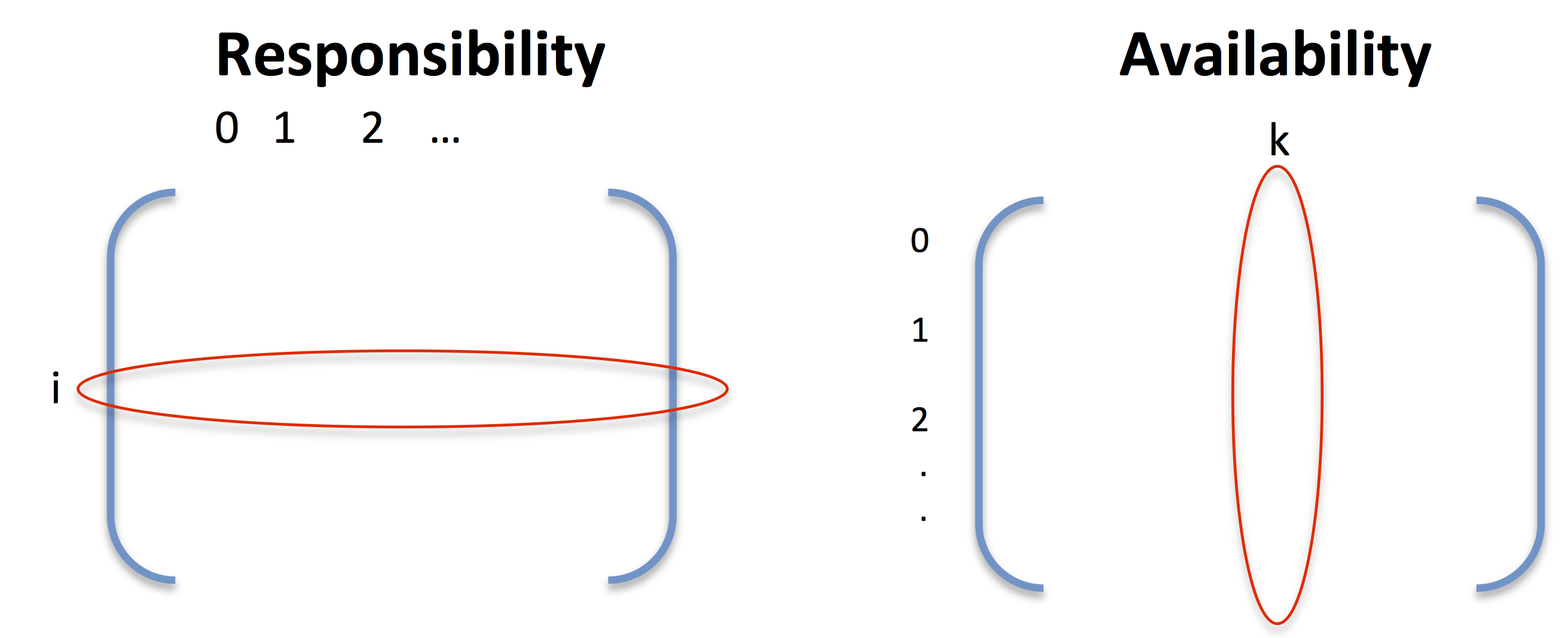
• responsibility, r(i, k) : A ‘message’ sent from point $i$ to point $k$ judging how well point $k$ will be a suitable exemplar for point $i$ taking in to account other potential exemplars.
• availability, a(i, k) : A ‘message’ sent from point $k$ to point $i$ judging how appropriate $i$ should choose $k$ as an exemplar, taking in to account other points $k$ should represent.

More formally, the availibility and responsibility are defined as follows:

Let’s talk through these for a second. The responsibility, $r(i, k)$ can be thought of as $i$ trying to see how well $k$ would be as its representative. It first considers how similar $i$ is to $k$. This is balanced by seeing how similar $i$ is to all the other points as well as how well these other points would represent it. The availability, $a(i, k)$ is somewhat the opposite and is defined separately for $i=k$ and $i \neq k$. The availibility for $i \neq k$ considers how good point $k$ would be representing itself as well as every other point. This is capped off using the maximum of {0, value} because we only care about the values for which $k$ is a good exemplar. The larger the value, the more likely $k$ is as being a suitable exemplar. Note that the final $\min$ is just to ensure large responsibilities do not skew the values. For $i=k$, the availability $a(k, k)$ looks at how well point $k$ is a representative for all other points. Again, we only care about the positive values because we only care about when $k$ is a good representative. If the ideas are still fuzzy, check out Frey and Deuck’s paper. They go throught this in more detail and in plain easy old English.

It might be helpful to think of responsibility as iterating over columns and availability as iterating over rows.

A couple of technical details to keep in mind is that $a(i, k)$, $r(i, k)$ are initially set to 0 for all $i, k$, and that a damping factor is added to $r(i, k)$ and $a(i, k)$ to avoid oscillations.

Getting the Exemplars:

At any iteration we get the exemplars (or centroids) using the following

That is, the exemplar or representative for observation $i$ is the observation that maximizes the sum of the availbility and responsibility of $i$.

Example

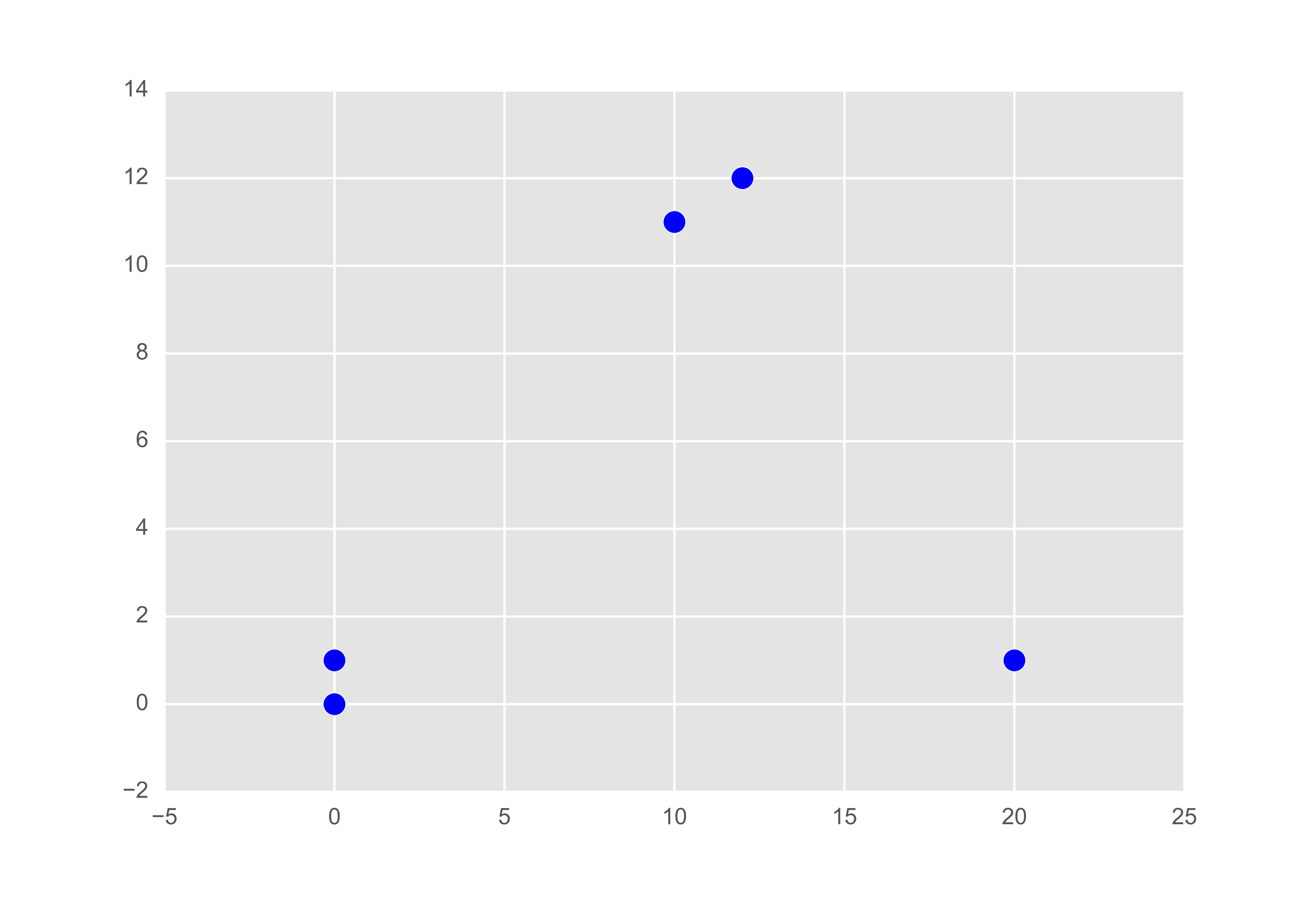
If you’ve managed to stick around so far, you deserve an example. Let’s consider a sample of five data points:

If we plot it out we might imagine what the partition might be like. Of course the scale of the plot may skew our thoughts, but let’s see what the algorithm tells us.

Let’s compute the similarity matrix using $s(i, j) = - |x_i - x_j|^2$ as per Frey and Dueck.

Recall that $diag(S), s(k, k)$ is the ‘preference’ of point $k$. The suggested default is the median of $S$ so let’s go ahead and redefine $S$ with this value for $s(k, k)$.

Let’s also go ahead and compute the first iteration of the responsibility, $R$ and availability, $A$. matrices. (Recall that initially, we set $R \equiv 0$ and $A \equiv 0$).

As example calculations, we’ll compute $r(2, 3)$,

and $a(2, 3)$,

These are 0 indexed matrices so that the top left corner is the (0, 0) entry and the (2, 3) entries are highlighted in red. Then,

and

If we were to stop the algorithm here, what would be our exemplars? Recall that the exemplar for observation $i$ is given by \(E(i) = argmax_{k} \, a(i, k) + r(i, k).\) That is, in computing the sum of $A$ and $R$, for each observation (row), we find the index of the maximum value:

So here we have three exemplars: 0, 1, and 2.

${\color{red} 0}$: Represents 1 and 3

${\color{red} 1}$: Represents 0

${\color{red} 2}$: Represents 2 and 4

It is interesting to see that although 0 and 1 are exemplars, they do not represent themselves.

Now let’s see what happens after 100 iterations. Below is a plot of the clusters (colour coded) after 1 and 100 iterations.

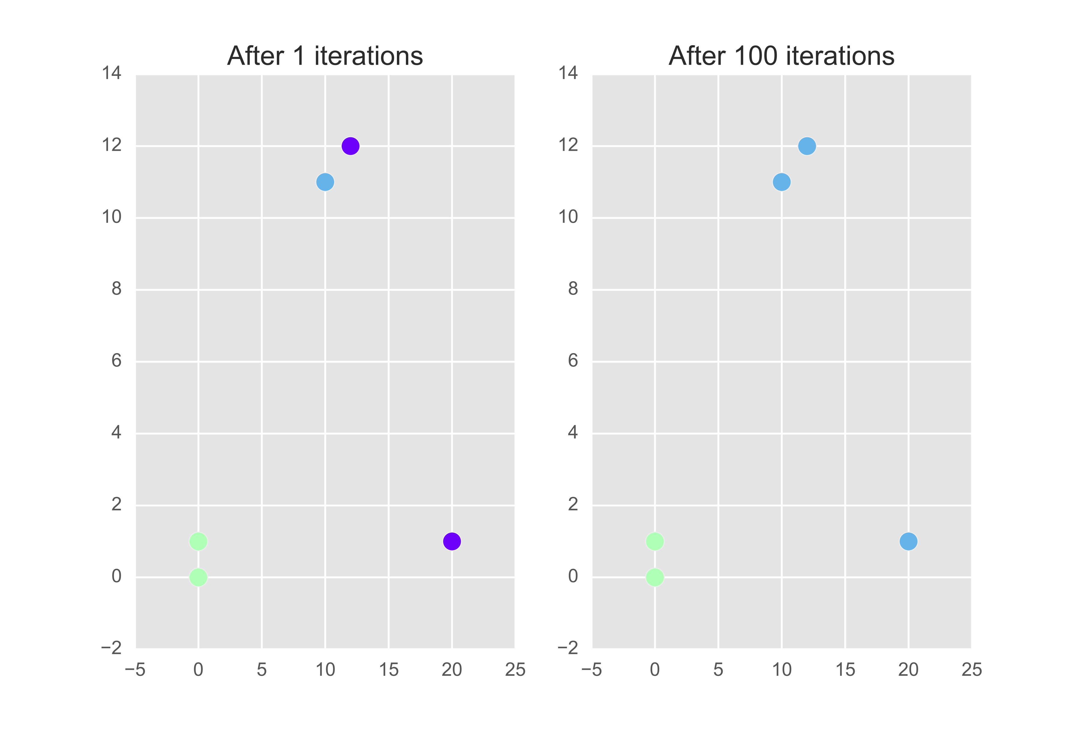
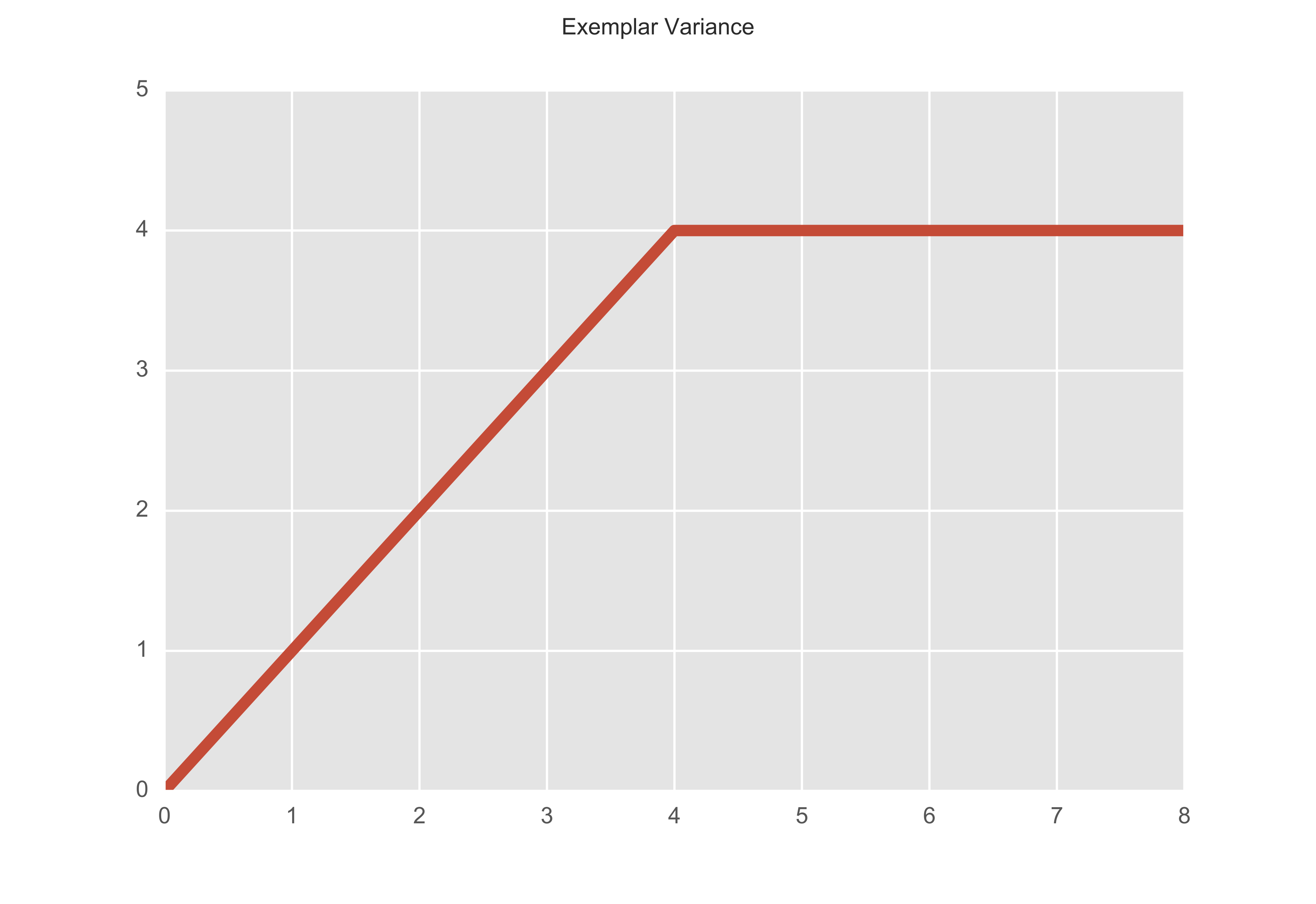
How do we actually know when we should stop? Well let’s take a look at how often these assignments actually change. We can record anytime there is any change of assignments in each iteration. In the plot below, we increase the step by 1 every time there is a change. In 100 iterations, the exemplar assignments changed at the 5th and 6th iteration, and remained constant thereafter.

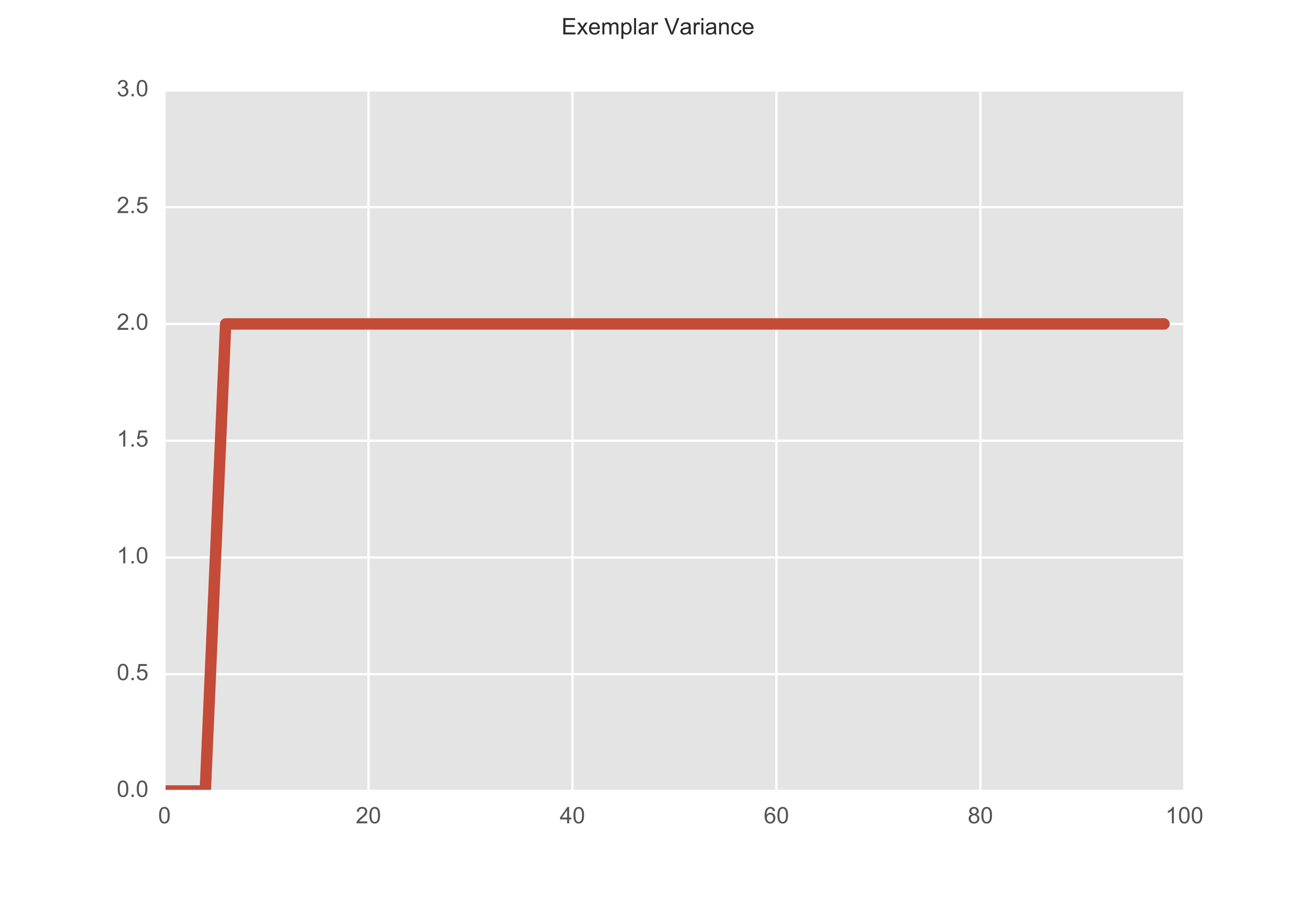
We can choose our stopping point to be the assignments after there is no change in $x$ iterations, say, where $x$ is a number we choose beforehand.

Let’s explore the preference parameter with a slightly more meaningful example.

Preference

Below, again, I have randomly generated some points, colour coordinated to represent my intuitive clusters, based on the scale of my plots.

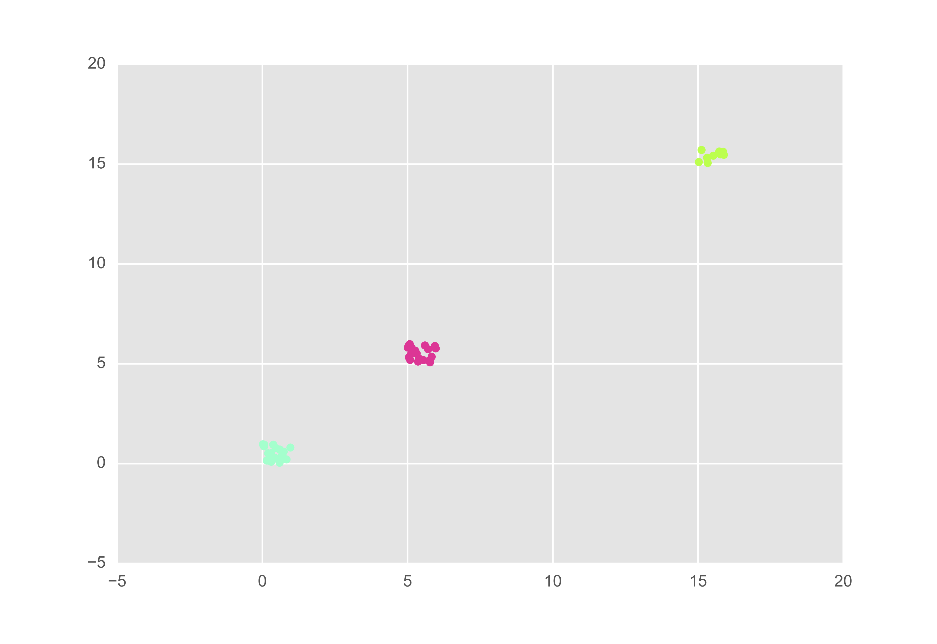
Recall that the larger the preference, $s(k, k)$, the more inclined observation $k$ is to be an exemplar. Thus, as expected, if we assign $s(k, k) = 0$ for all $k$, each point becomes its own exemplar. This is represented in the figure below although it may be hard to decipher that each point is in fact distinctly coloured.

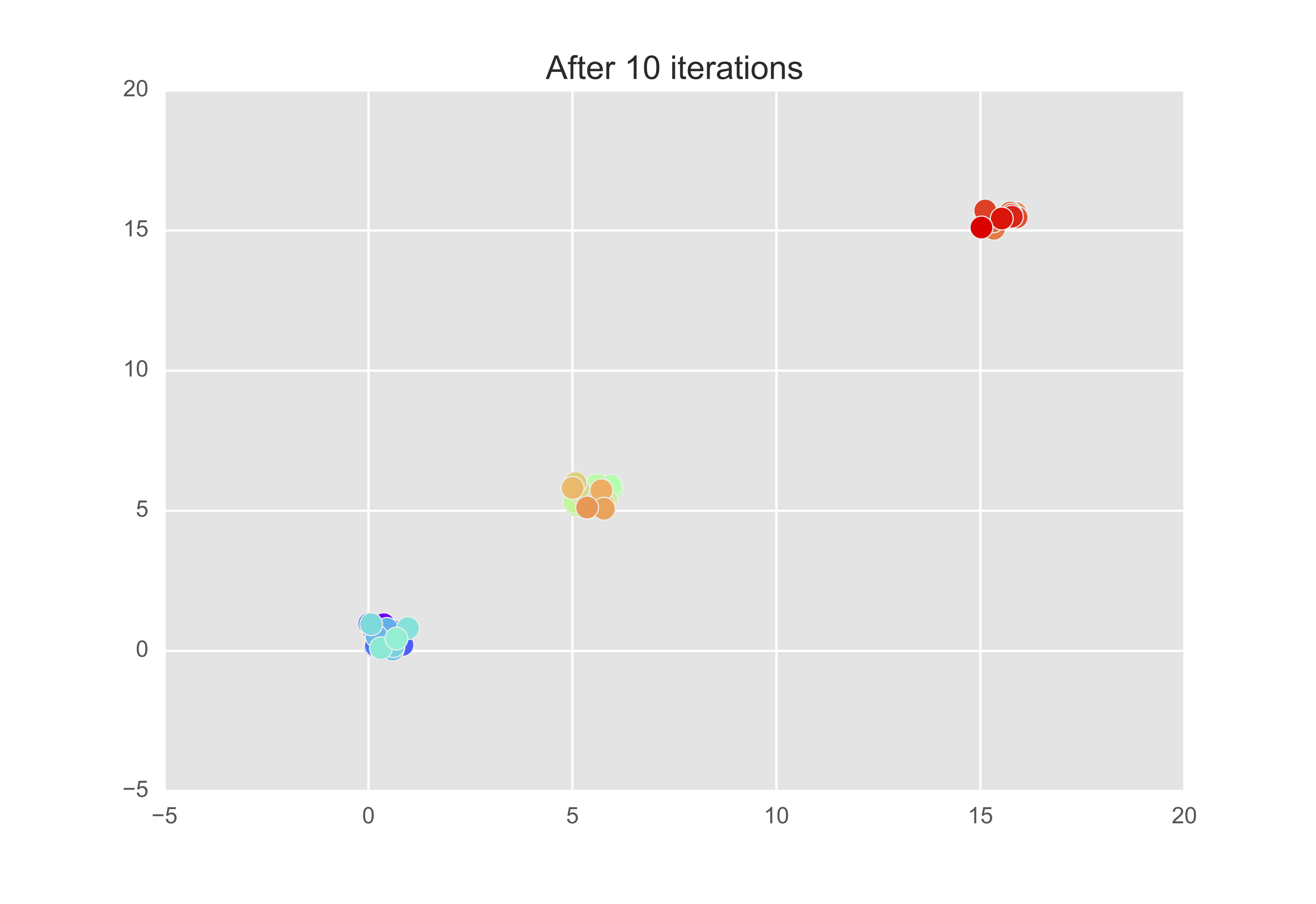
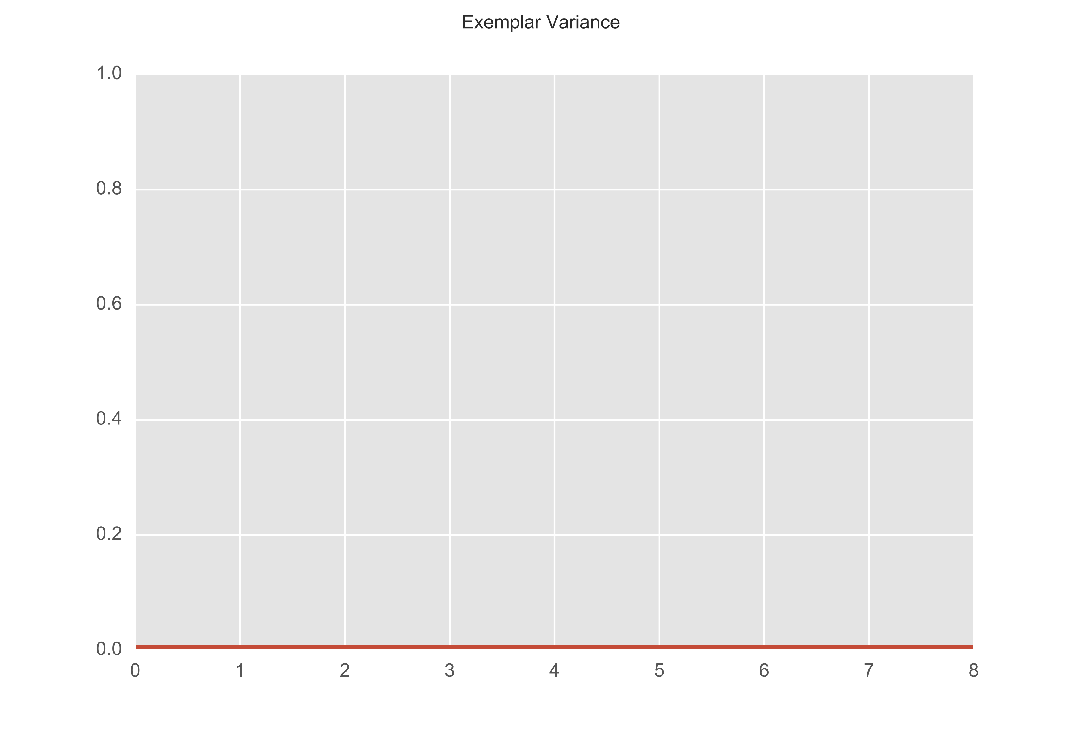
This is the output after only 10 iterations but we can see that there is no variance on the output (recall we increase the y value by one every time there is a change.)

Let’s now change the preference so that $s(k, k) = $ minimum of the similarity matrix. Then after 10 iterations, we get that there are indeed 3 exemplars - observations 8, 28, and 49.

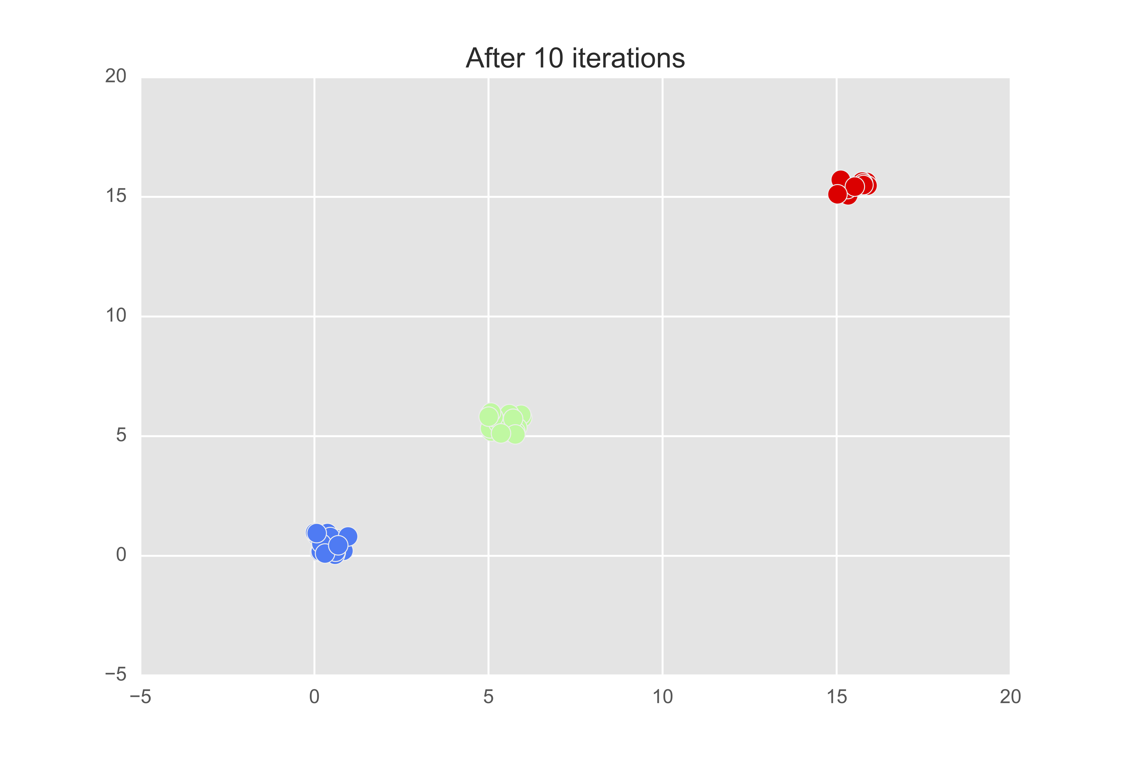
The assingments changed up to the fourth iteration but then remained constant.

As you can see, the preference parameter is the influencing factor in the total number of outputted clusters. So although we do not need to specify the number of clusters to run the algorithm, we can, in some, sense, give preference to certain observations over others, in becoming exemplars.

Summary

The affinity propagation algorithm is a useful unsupervised learning algorithm that allows the algorithm to naturally deduce the number of clusters, given the similiarity of each observation to one another, and the likelihood the observation will be an exemplar. I hope this introductory piece supplements B. Frey’s and D. Dueck’s paper with a few more examples, providing a bit more detail on some of the computations.